Go to the table of contents

As network complexity increases, graphical representations become cluttered and difficult to interpret. Osprey simplifies network layouts through user implemented node relaxation, which disperses nodes and edges according to any one of a number of layout options. Any given node or set of nodes can be locked into place in order to anchor the network. Osprey also provides several default network layouts including:

1. One Circle (section 6.2.1 One Circle)
2. Concentric (section 6.2.2 Concentric Circles)
3. Dual Ring (section 6.3 Dual Ring Layouts)
4. Spokes (section 6.4 Spokes)
5. Spoked Dual Ring (section 6.5.1 Spoked Dual Ring)

The auto relaxation method attempts to place the nodes in the graph at a pre-defined distance from each other without intersecting any lines. This iterated relaxation results in a more easily viewable graph (The auto relaxation method is an extension of the Java Sun graphing algorithm version 1.8 98/10/28 which can be found at http://java.sun.com).

Note: When "Start Relax "is called it will continue relaxing the nodes until"Stop Relax"is called.

Section 6.1.1 Accessing the auto relaxation from the main menu demonstrates the ways in which to activate the auto relaxation method.

There are currently two ways in which the user can access the auto relaxation method:

1) The Menu Bar

• Select all nodes that need to be relaxed
• Click on the "Layout" overhead menu
• Click on the "Auto Relaxation" submenu
• Click on "Start Relax", see figure 6.1.1 - 1
• To Stop the relaxation process follow the same steps as above and click on "Stop Relax"

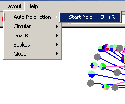
Figure 6.1.1-1 Accessing the relaxation method via the main menu

Note: The other way to stop is to click the small stop button at the bottom right hand corner of the screen (this button is only active when the graph is being relaxed) see figure figure 6.1.1-2.

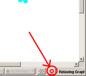
Figure 6.1.1-2 Stop relaxation button

2) Hot Key (ctrl + R)

• Select all nodes that need to be relaxed
• Click the ctrl + R buttons together on your keyboard to start relaxation
• Click the ctrl + R buttons again to stop relaxation
• The other way to stop is to click the small stop button at the bottom right hand corner of the screen (see Figure 6.1.1-1)

The circular layouts place the selected nodes in either a single circle or concentric circles. The concentric circles function can be adjusted in advanced settings to achieve the best look for each situation.

Note: The radii of the circles depends on the size of the selection box created with the mouse before calling these functions. If all the Nodes on the screen are selected this gets overridden and the radii become as large as possible in the current graph size. If the function call is repeated the diameter will increase until the maximum graph width and height are reached.

This layout is used to position the selected nodes in one circle. There are 2 ways to call this function, see section 6.2.1.1 Accessing the one circle layout for details.

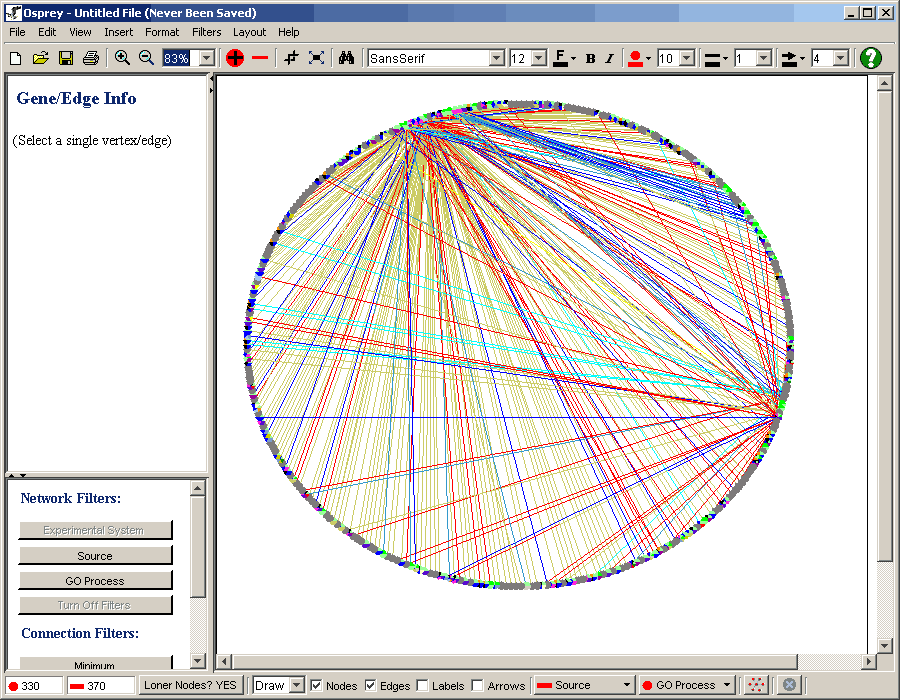
Figure 6.2.1-1 Network layout out using the one circle method

There are currently two ways in which the user can access the one circle layout:

1) The Menu Bar

• Select all nodes that you want in a circle
• Click on the "Layout" overhead menu
• Click on the "Circular" submenu
• Click on "One Circle"

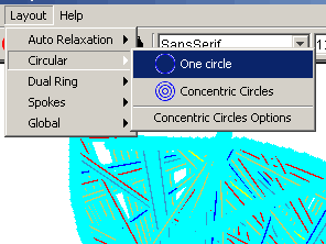
Figure 6.2.1-1 Accessing the one circle layout via the main menu

2) Right-Click Menu

• Select all nodes that you want in a circle
• Right click in an empty area of the graph
• Click on "One Circle Layout"

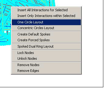
Figure 6.2.1-2 Accessing the one circle layout via the Right-Click Menu

This layout is used to position the selected nodes in a customizable number of concentric circles. Figure 6.2.2-1 demonstrates a network layout using the concentric circles layout with 6 rings. For details on the options available for customizing the concentric circles see section 6.2.3 Concentric Circles Options.

There are 2 ways to call this function, see section 6.2.2.1 Accessing the Concentric Circles Layout for details.

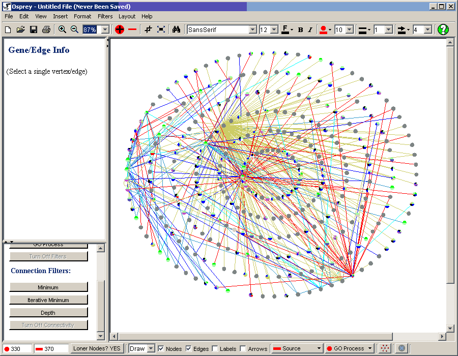
Figure 6.2.2-1 Example of the Concentric circles layouts with 6 rings

There are currently two ways in which the user can access the concentric circle layout:

1) The Menu Bar

• Select all nodes that you want in concentric circles
• Click on the "Layout" overhead menu
• Click on the "Circular" submenu
• Click on "Concentric Circles"

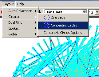
Figure 6.2.2-1 Accessing the concentric circles layout via the main menu

2) Right-Click Menu

• Select all nodes that you want in a circle
• Right click in an empty area of the graph
• Click on "Concentric Circles Layout"

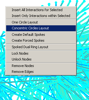
Figure 6.2.2-2 Accessing the concentric circles layout via the Right-Click Menu

Using the concentric circles options found in the Advanced Settings window under the tab labeled "Concentric Circles" (Figure 6.2.3-1 label #1) it is possible to adjust the the following settings:

1) Number of rings (Figure 6.2.3-1 label #2)

This adjusts the total number of concentric circles you want to place your selected nodes in.

2) Size of rings (Figure 6.2.3-1 label #3)

• This adjusts the radius of the smallest ring as a percentage of the largest ring.
• The distance between every ring larger than the smallest is divided equally

3) Capacity of rings (Figure 6.2.3-1 label #4)

• This adjusts the capacity of the smallest ring as a percentage of all nodes currently selected
• The remaining percentage of nodes is divided in an increasing manner so that the larger the ring the higher the percentage of nodes

  Note: if the percentage is too high to be able to place the remaining nodes in the selected number of rings, the largest possible percentage will be applied to the graph

Any changes made to the concentric circles options can be applied to the selected nodes by pressing the "Apply to selected nodes" button seen in figure 6.2.3-1 label #5.

There are two ways to access the concentric circles options, see section 6.2.3 Concentric Circles Options.

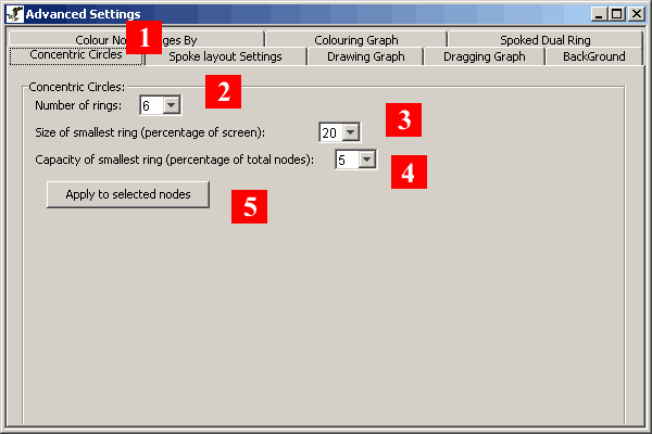
Figure 6.2.3-1 Concentric Circles advanced options tag

There are currently two ways in which the user can access the concentric circle options:

1) The Menu Bar

• Click on the "Layout" overhead menu
• Click on the "Circular" submenu
• Click on "Concentric Circles Options"

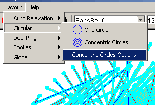
Figure 6.2.3-1 Accessing the concentric circles options via the main menu

2) Right-Click Menu

• Click on the "Format" overhead menu
• Click on "Advanced Settings"
• Look for the "Concentric Circles" tab and click on it

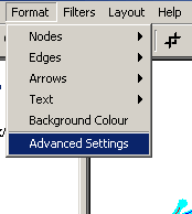
Figure 6.2.3-2 Accessing the concentric circles options via the Right-Click Menu

The dual ring layouts pick out the most highly connected nodes and place them in one ring (either in the inner ring or the outer ring depending on your selection) and place all the other nodes in the other ring.

Note: The radii of the circles depends on the size of the selection box created with the mouse before calling these functions. If all the Nodes on the screen are selected this gets overridden and the radii become the largest that can fit on the viewable area of your screen.

Follow the simple steps below to run either the "Highly Connected In" or "Highly Connected Out" Dual Ring Layouts:

• Select all nodes that you want in the Dual Ring Layout
• Click on the "Layout" overhead menu
• Click on the "Dual Ring" submenu
• Click on "Highly Connected In" (Figure 6.3-1) or the "Highly Connected Out" (Figure 6.3-2) option

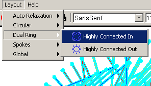
Figure 6.3-1 Main menu location of the highly connected in dual ring layout

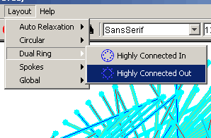
Figure 6.3-2 Main menu location of the highly connected out dual ring layout

Figure 6.3-3 demonstrates a network with a highly connected in layout, and figure 6.3-4 demonstrates a network with a highly connected out layout.

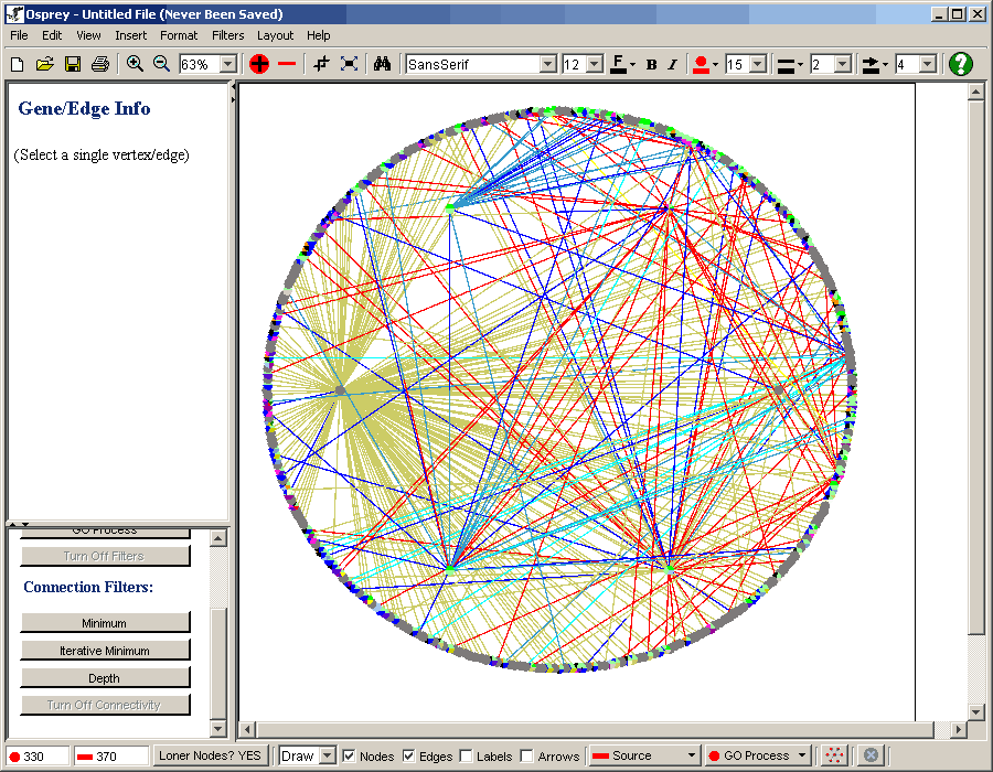
Figure 6.3-3: Dual Ring layout with the highly connected nodes in the inner ring

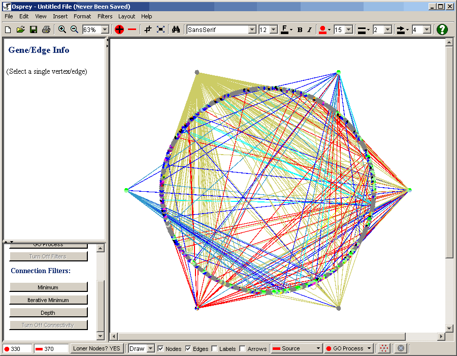
Figure 6.3 - 4: Dual Ring layout with the highly connected nodes in the outer ring

The Spokes layout attempts to take a selected nodes interacting partners and lay them out in a circular fashion up to three ring deep (The Spokes name comes from the resemblance of the spokes in a wheel). Osprey currently supports two different types of Spoked layouts:

1. Default Spokes (section 6.4.1 Default Spokes)
2. Forced Spokes (section 6.4.2 Forced Spokes)

Default spokes circles up all nodes that are connected except nodes that are centers of other spokes and nodes that are shared between two spoke models. Figure 6.4.1-1 demonstrates 5 default spoke models separated by the colours: red, green, grey, blue and yellow. The nodes coloured in purple are those that are connected to two or more spoke models and thus have not been placed in one of the rings of a spoke to allow the user to easily see highly connected nodes.

There are two ways to call the default spokes function, see section 6.4.1.1 Accessing the default spoke model.

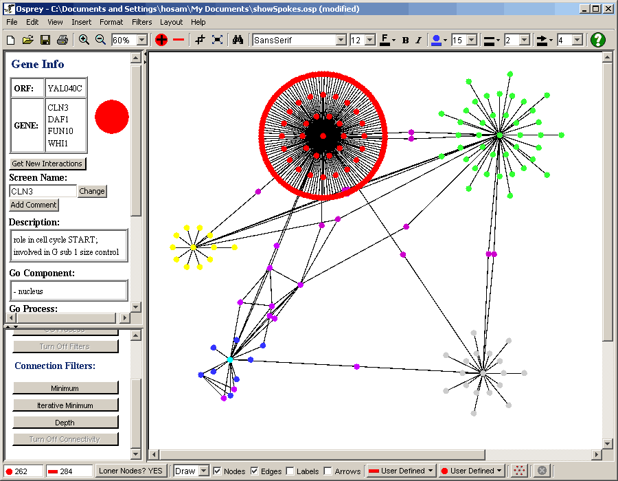
Figure 6.4.1-1 Default Spoke Models

There are currently two ways in which the user can access the default spoke model:

1) The Menu Bar

• Select all nodes that you want to be in the centers of default spokes
• Click on the "Layout" overhead menu
• Click on the "Spokes" submenu
• Click on "Default"

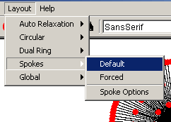
Figure 6.4.1.1-1 Accessing the default spokes layout via the main menu

2) Right-Click Menu

• Select all nodes that you want to be in the centers of default spokes
• Right click in an empty area of the graph
• Click on "Create Default Spokes"

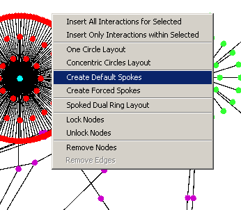
Figure 6.4.1.1-2 Accessing the default spokes layout via the Right-Click menu

Forced spokes bring in all nodes that are connected to the selected node into a spoke model. By comparing the blue and purple nodes in figures 6.4.2-1 and 6.4.1-1 you can see the difference between the default and forced spokes method. The nodes coloured purple represent nodes that share interactions with more than one spoke model, in the default spoke method these nodes would not get circled up into on of the three possible rings. But in the forced spoked model all interactions are treated the same and therefore the purple ones get added to the rings of the blue spoke model seen in figure 6.4.2-1.

There are two ways to call the forced spokes function, see section 6.4.2.1 Accessing the forced spoke model for details.

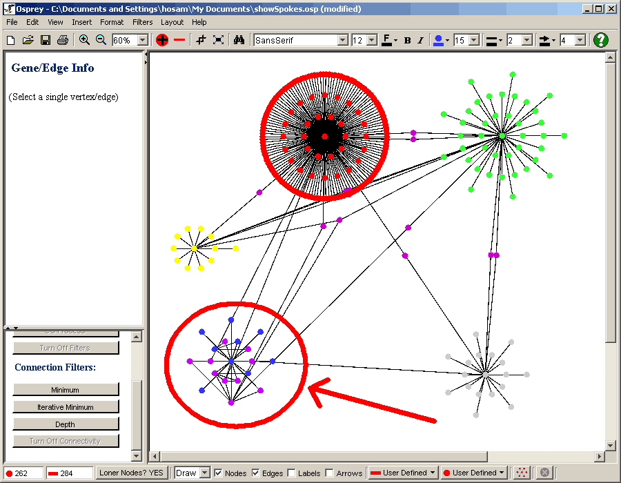
Figure 6.4.2-1 Forced Spoked Models

There are currently two ways in which the user can access the default spoke model:

1) The Menu Bar

• Select all nodes that you want to be in the centers of forced spokes
• Click on the "Layout" overhead menu
• Click on the "Spokes" submenu
• Click on "Forced"

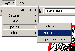
Figure 6.4.2.1-1 Accessing the forced spokes layout via the main menu

2) Right-Click Menu

• Select all nodes that you want to be in the centers of forced spokes
• Right click in an empty area of the graph
• Click on "Create Forced Spokes"

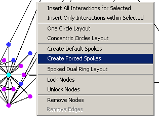
Figure 6.4.2.1-2 Accessing the forced spokes layout via the right click menu

Using the spoke options found in the Advanced Settings window under the tab labeled "Spoke layout Settings" (Figure 6.4.3-1 label #1) it is possible to adjust the the following settings:

1) Size of smallest ring (Figure 6.4.3-1 label #2)

• This adjusts the radius of the smallest ring as a percentage of the largest ring.
• The distance between every ring larger than the smallest is divided equally

2) Capacity of smallest ring (Figure 6.4.3-1 label #3)

• This adjusts the capacity of the smallest ring as a percentage of all nodes currently selected
• The remaining percentage of nodes is divided in an increasing manner so that the larger the ring the higher the percentage of nodes

There are two ways to access the concentric circles options, see section 6.4.3.1 Accessing the spoke options.

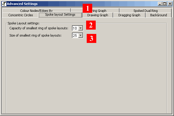
Figure 6.4.3-1 Spoke layout settings advanced options tag

There are currently two ways in which the user can access the spoke options:

1) The Layout option in the Menu Bar

• Click on the "Layout" overhead menu
• Click on the "Spokes" submenu
• Click on "Spoke Options"

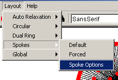
Figure 6.4.3.1-1 Accessing the spokes options via the main menu

2) The Advanced settings options in the Menu Bar

• Click on the "Format" overhead menu
• Click on "Advanced Settings"
• Look for the "Spoke Settings" tab and click it

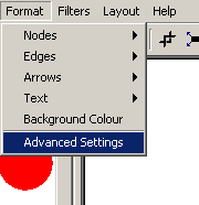
Figure 6.4.3.1-2 Accessing the spokes options via the main menus advanced settings under the Format menu

By global we mean that these layouts will be applied to all visible (unfiltered) nodes. These layouts will ignore any locks that are currently on nodes and it does not matter what nodes are currently selected, these algorithms are applied to all nodes. The current graph size will also be adjusted to best fit the nodes.

This function places the most highly connected spokes (customizable minimum) in the inner spoked ring. It places the less highly connected spokes (customizable minimum) in the outer spoked ring and it relaxes all nodes that are shared between two or more nodes to the center of mass position where all shared spoke centers are an equal distance away, see figure 6.5.1-1.

There are two ways to call this function, see section 6.5.1.1Accessing Spoked Dual Ring Layout for details.

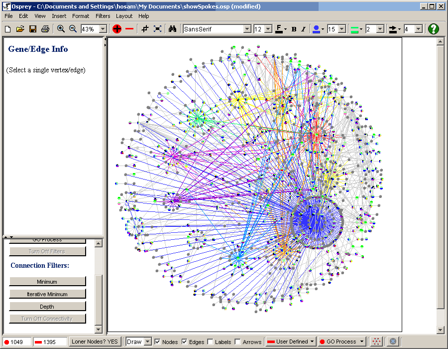
Figure 6.5.1-1 Network demonstrating the Spoked Dual Ring layout

There are currently two ways in which the user can access Spoked Dual Ring Layout Option:

1) The Layout option in the Menu Bar

• Click on the "Layout" overhead menu
• Click on the "Global" submenu
• Click on "Spoked Dual Ring"

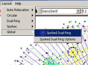
Figure 6.5.1.1-1 Accessing the spoked dual ring via the main menu

2) Right-Click Menu

• Right click in an empty area of the graph
• Click on "Spoked Dual Ring"

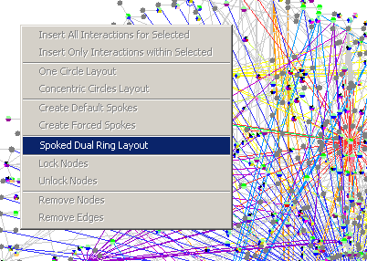
Figure 6.5.1.1-2 Accessing the spoked dual ring via the right-click menu

Using the Spoked Dual Ring Options found in the Advanced Settings window under the tab labeled "Spoked Dual Ring" (Figure 6.5.2-1 label #1) it is possible to adjust the the following settings:

1) Min Edges for spokes in INNER ring (Figure 6.5.2-1 label #2)

• This sets the minimum cutoff for the number of connected free nodes required for a spoke to be in the INNER ring
• Anything less than this cutoff will be in the outer ring

2) Min Edges for spokes in OUTER ring (Figure 6.5.2-1 label #3)

• This sets the minimum cutoff for the number of connected free* nodes required for a spoke to be in the OUTER ring
• Anything less than this cutoff will not make it to either ring. It will relaxed somewhere on the screen

3) Size of smallest spoke ring (Figure 6.5.2-1 label #4)

• This adjusts the radius of the smallest ring as a percentage of the largest ring.
• The distance between every ring larger than the smallest is divided equally

4) Capacity of smallest spoke ring (Figure 6.5.2-1 label #5)

• This adjusts the capacity of the smallest ring as a percentage of all nodes currently selected
• The remaining percentage of nodes is divided in an increasing manner so that the larger the ring the higher the percentage of nodes

There are two ways to access the Spoked Dual Ring Options, see section 6.5.2.1 Accessing Spoked Dual Ring Layout Option settings.

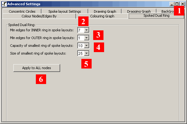
Figure 6.5.2-1 Spoked dual ring layout settings advanced options tag

There are currently two ways in which the user can access Spoked Dual Ring Layout Option settings:

1) The Layout option in the Menu Bar

• Click on the "Layout" overhead menu
• Click on the "Global" submenu
• Click on "Spoked Dual Ring Options"

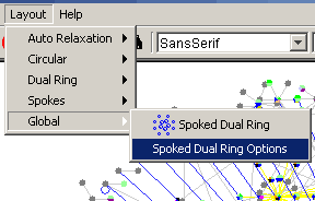
Figure 6.5.2.1-1 Accessing the spoked dual ring layout options via the main menu bar under the Layout menu

2) The Advanced settings options in the Menu Bar

• Click on the "Format" overhead menu
• Click on "Advanced Settings"
• Look for the "Spoked Dual Ring" tab and click it

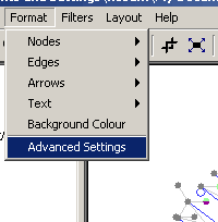
Figure 6.5.2.1-2 Accessing the spoked dual ring layout options via the main menu bar under the Format menu

Osprey has the ability to cluster genes by their GO Process. When any of the layouts discussed above (except the Dual ring layouts) are invoked, nodes that have a common Go Process will be grouped together. When nodes have multiple Go Processes they are put in the group with the highest order GO Process. This GO Process Order can be adjusted in Advanced Settings which is discussed is section 6.6.2 GO Process Ordering below. To make clusters easier to see, there are empty gaps between them. The gap size can be adjusted or taken out completely, how to do this is discussed below in section 6.6.3 Cluster Gap Size.

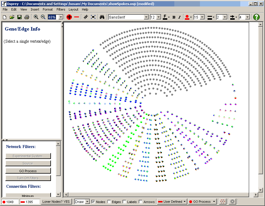
Figure 6.6-1 Concentric Circles with Functional Clustering turned on

Functional Clustering can be turned on or off under the "Functional Clustering" heading in Advanced Settings. Follow these steps to find out exactly how to do so:

The Advanced settings options in the Menu Bar

• Click on the "Format" overhead menu
• Click on "Advanced Settings"
• Look for the "Functional Clustering" tab and click it

Figure 6.6.1-1 Accessing Functional Clustering options via the main menu bar under the Format menu

The GO Processes can be ordered in terms of importance so that if a node is classified under several GO Processes it will be clustered with the most important one. After accessing the Functional Clustering menu described in section 6.6.1 Accessing Functional Clustering options, the next few steps will explain how the ordering is done:

1) Moving a "GO Process" down the list:

• Click on the desired GO Process
• Either drag it down to the desired order
• Or click the down arrow (moves down one step at a time)

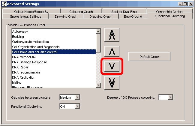
Figure 6.6.2-1 Move down the list

• Note: to move all the way down click the "bottom" button

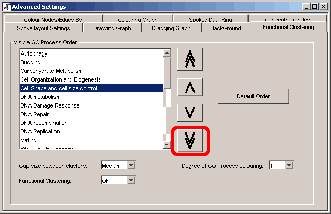
Figure 6.6.2-2 Move to the bottom of the list

 

 

2) Moving a "GO Process" up the list:

• Click on the desired GO Process
• Either drag it up to the desired order
• Or click the up arrow (moves down one step at a time)

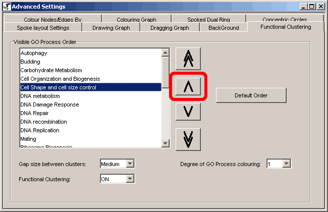
Figure 6.6.2-3 Move up the list

• Note: to move all the way up click the "top" button

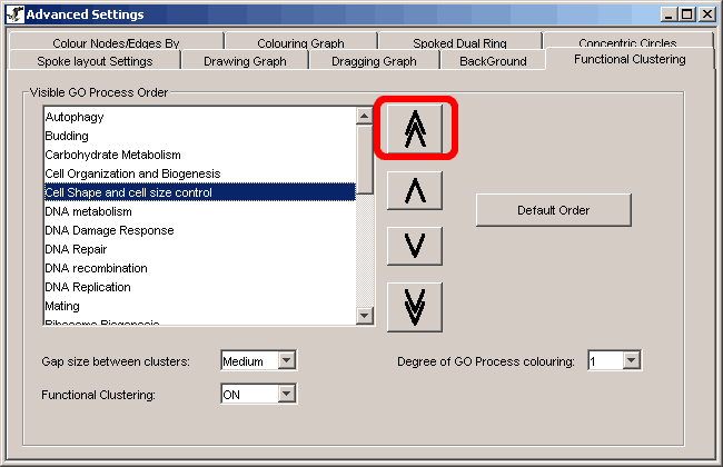
Figure 6.6.2-4 Move to the top of the list

After accessing the Functional Clustering menu described in section 6.6.1 Accessing Functional Clustering options follow these steps to create a smaller or larger gap that seperates the clusters in a layout:

• Choose the desired gap size, or none for no gap at all

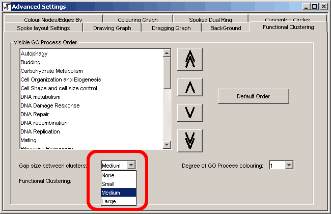
Figure 6.6.3-1 Choosing Gap size

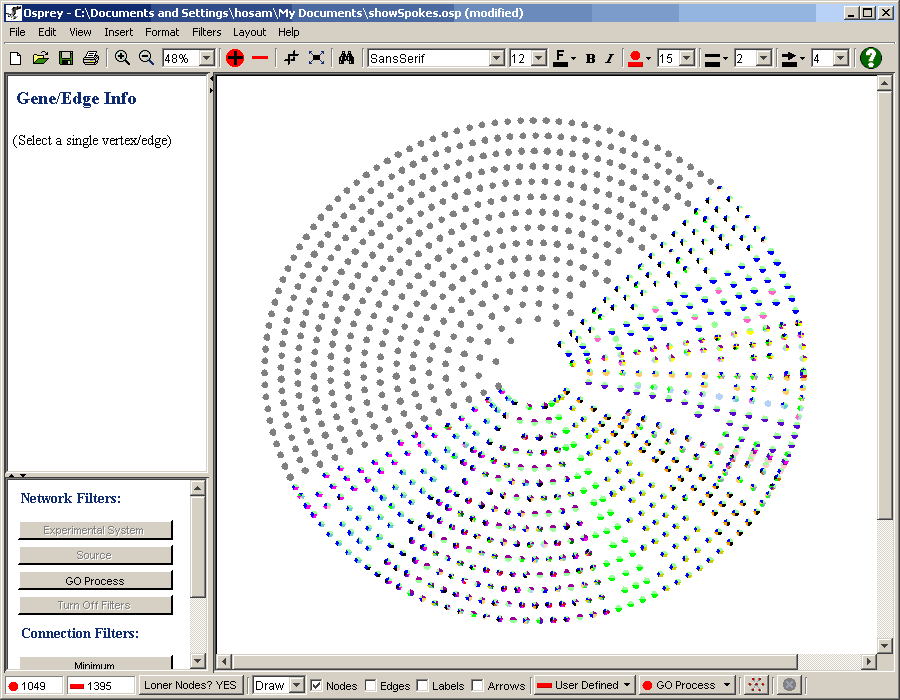
Figure 6.6.3-2 Concentric Cicrcles with no gap

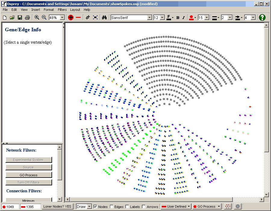
Figure 6.6.3-3 Concentric Cicrcles with large gap

After accessing the Functional Clustering menu described in section 6.6.1 Accessing Functional Clustering options, follow these steps:

• Click on the drop down box shown below to turn it on or off.
• Note: you will have to perform the layout again to see a change

 

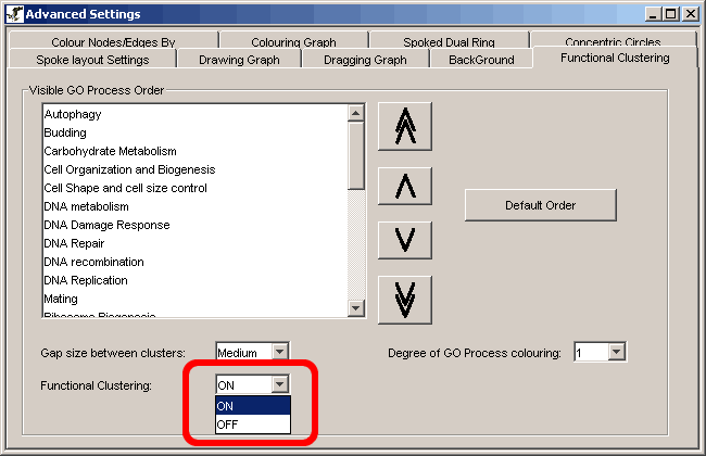
Figure 6.6.1-2 Turning Functional Clustering on/off

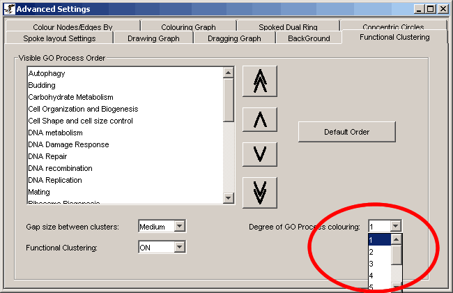
Figure 6.6.5-1 Degree of GO Process colouring



Figure 6.6.5-2 Network with a degree of GO Process colouring of 1



Figure 6.6.5-2 Network with a degree of GO Process colouring of 3

The Osprey Administrator

E-mail: ospreyadmin@mshri.on.ca

Go to the table of contents